Overview
The Frequency -> Time Task
This section deals with the task of creating time-domain signals out of individual sinewave components in the frequency domain.
First, download this Fourier example file and load it into Maxima. It contains a set of example functions that show aspects of Fourier analysis.
In this section we'll be using Maxima to build complex waveforms out of simple components. To reiterate, any signal can be built out of individual sinewave components, arranged in particular ways. Remember this the next time you're listening to your favorite music — in principle, it can be created out of a mathematical description consisting only of sinewave frequencies, amplitudes and phases.
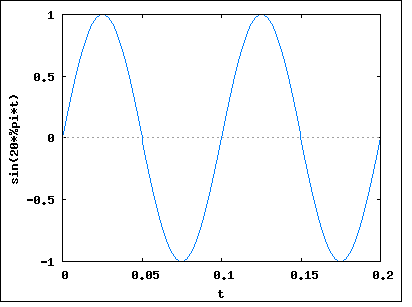
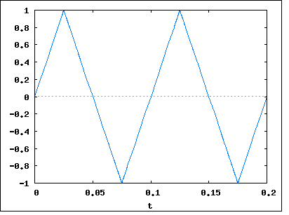
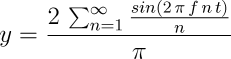
Let's begin with a table of classic wave equations and corresponding graphs:
Obviously these graphs weren't created by summing
terms from 1 to ∞ as indicated by the equations in the left column. In
practice one chooses a summation number that balances display quality
with a reasonable running time. But by choosing different upper bounds
for these summations, we can learn something important about signal
generation.
Make sure you have loaded this Fourier examples file into Maxima, then enter this at the keyboard:
In case it isn't obvious from the equation listed above, the square wave is created by accumulating the odd multiples of a specified frequency — in this way (where x = 2 π f t):
The Fourier examples file contains a set of waveform generating functions, one for each kind of waveform in the above table. Here are their names:
Here is a list of the multiple-plot functions:
In this section we'll be using Maxima to build complex waveforms out of simple components. To reiterate, any signal can be built out of individual sinewave components, arranged in particular ways. Remember this the next time you're listening to your favorite music — in principle, it can be created out of a mathematical description consisting only of sinewave frequencies, amplitudes and phases.
Let's begin with a table of classic wave equations and corresponding graphs:
| Name | Equation | Graph |
| Sine |
|
|
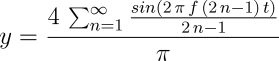
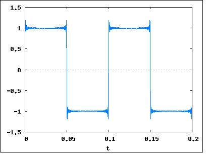
| Square |
|
|
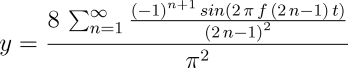
| Triangle |
|
|
| Sawtooth |
|
|
| Rectified Sine |
|
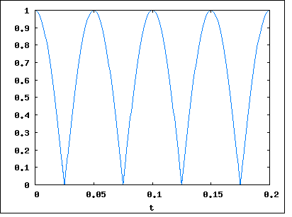
|
Make sure you have loaded this Fourier examples file into Maxima, then enter this at the keyboard:
fpsq(1);This will accumulate one element from the square-wave equation, which, if you think about it, must be a sine wave (because all these generators use individual sine waves as their building blocks). Now change your entry to this:
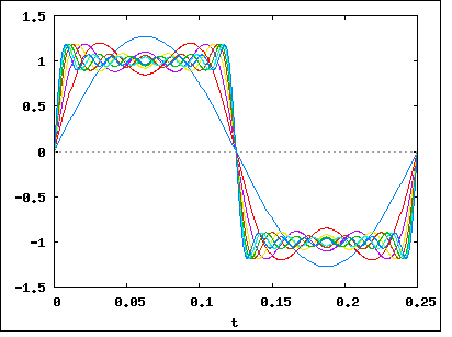
fpsq(2);Notice the difference. Now change the number, go as high as you like, considering the issue of running time, and see how the plotted wave changes. You will begin to see a pronounced "ringing" transient at the switching points in the waveform (like the graph on this page), and the ringing will become more severe as the number of accumulations increases. There is a longstanding debate among mathematicians as to whether this ringing is an artifact of our imperfect generation methods or a real property of square waves.
In case it isn't obvious from the equation listed above, the square wave is created by accumulating the odd multiples of a specified frequency — in this way (where x = 2 π f t):
y = (4/π) (sin(x) + 1/3 sin(3x) + 1/5 sin(5x) + 1/7 sin(7x) ...)These sine terms are combined to create the time-varying waveform in the display. And if the opposite operation were to be performed on the result (something called a Fourier transform), these individual harmonic elements would reappear. It is important to reemphasize that waveform generation, and the Fourier transform, are reciprocal operations. You can use frequency components to generate a waveform in the time domain, then transform the result back to the frequency domain and recover what you started with. This reciprocal relationship is to Fourier analysis what the Fundamental Theorem of Calculus (the idea that integration and derivation are reciprocal operations) is to Calculus.
The Fourier examples file contains a set of waveform generating functions, one for each kind of waveform in the above table. Here are their names:
- fpsq(n); (square)
- fptri(n); (triangle)
- fpsaw(n); (sawtooth)
- fprec(n); (rectified sine)
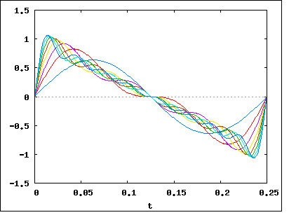
| Function | Graph |
| fsqmult(8); |
|
| fsawmult(8); |
|
- fsqmult(n); (square)
- ftrimult(n); (triangle)
- fsawmult(n); (sawtooth)
- frecmult(n); (rectified sine)
The Time -> Frequency Task
Converting from the time domain to the frequency
domain is a bit more labor-intensive than the task of generating complex
waveforms, the topic covered above. The general name for this
conversion is "Fourier Transform", and because of its usefulness, much
thought and ingenuity have been expended on this task.
In the 1960s, an apparently new and much more efficient method for this conversion, now called the "Fast Fourier Transform" (FFT), was devised by J. W. Cooley and John Tukey. I say "apparently" because it turns out the basic idea behind the FFT was developed by Carl Friedrich Gauss in 1805 and was rediscovered by others in various limited forms in the intervening years.
Maxima has an FFT package available, made accessible by loading a library named "fft". Here is an outline of the steps needed to perform an FFT in Maxima:
If everything is in order on your system and there is nothing wrong with your Maxima installation, the predicted and result data lists should be nearly identical. Because the FFT is a numerical procedure performed on machines with finite floating-pint resolution and a finite array size, all FFT results are approximate.
I want to emphasize that the numerical, approximate nature of the FFT doesn't imply that all Fourier transforms are approximate. The FFT is a specific, very fast, embodiment of a well-understood mathematical transformation that can be carried out analytically in some circumstances. What I am saying here is ... don't confuse the FFT with the field itself.
In the 1960s, an apparently new and much more efficient method for this conversion, now called the "Fast Fourier Transform" (FFT), was devised by J. W. Cooley and John Tukey. I say "apparently" because it turns out the basic idea behind the FFT was developed by Carl Friedrich Gauss in 1805 and was rediscovered by others in various limited forms in the intervening years.
Maxima has an FFT package available, made accessible by loading a library named "fft". Here is an outline of the steps needed to perform an FFT in Maxima:
There are example functions in the Fourier examples file that show a typical conversion:
load(fft); Load the required library. n:2048; Establish an array size, which must be:
- A power of 2 (512,1024,2048, etc.).
- Twice the size of the highest frequency of interest in Hertz, e.g. to resolve frequencies between 0 and N Hertz, the array size must be the next higher power of 2 above N * 2.
array(ra,float,n-1); Declare a real-value array. array(ia,float,n-1); Declare an imaginary-value array. for i:0 thru n-1 do ( Fill the array with the desired data. ra[i]:my_function(i), This is a user-defined function that is able to create suitable data. ia[i]:0.0 Must set the imaginary array to zero if there are no data. ); fft(ra,ia); Perform the FFT conversion in-place (the original array data are overwritten). recttopolar(ra,ia); Optional: convert complex a+bi form to polar magnitude and angle form. lira:makelist(ra[i],i,0,(n/2)); For plotting, create a list out of the first half of the data array. xIndexList:makelist(i,i,0,length(lira)); Create an index list required by the plotting routine. wxplot2d([discrete, xIndexList,lira], [gnuplot_preamble, "unset key;set xrange [0:1024];set xlabel 'Frequency';set ylabel 'Amplitude';set title 'Amplitude Modulation — Frequency Domain';"]); Create an inline plot (one that is integrated into wxMaxima's display).
There is one more experiment in the Fourier examples file. It is meant to clearly show the equivalence of time-domain and frequency-domain representations of spectral data. In this experiment, we will:
fpt(); 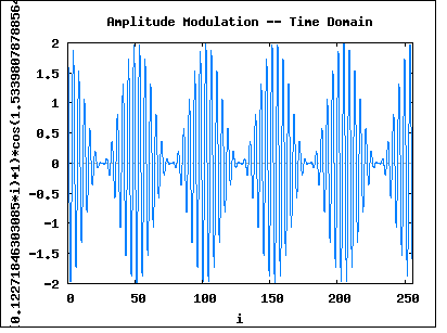
This time-domain plot shows a waveform that was once very familiar to electrical engineers: an amplitude-modulated (AM) radio signal. In the AM scheme, information is added to a radio carrier wave by changing its amplitude. Speaking mathematically, this modulation method creates sidebands whose distance from the carrier frequency is equal to the modulation frequency. Typically the modulation of a real-world AM radio signal is complex and broad. In this example, we're modulating the carrier with a simple sinewave.
This plot is the input data for the FFT. If you have loaded the Fourier examples file into Maxima, and if you enter the function name at the left, you will get this plot.
fpf(); 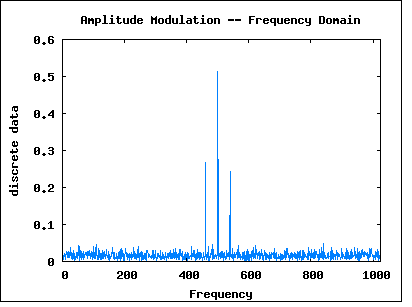
Here is the frequency-domain equivalent of the above time-domain plot (with some random noise added for a touch of realism). The central peak is the carrier frequency, and there are two sidebands, one above and one below the carrier frequency. The sideband frequencies are located at c+m and c-m, where c = carrier frequency and m = modulation frequency.
This plot is the output data from the FFT. If you have loaded the Fourier examples file into Maxima, and if you enter the function name at the left, you will get this plot.
- Create a square wave signal in the time domain using the methods established above,
- Convert the time-domain data back to the frequency domain using the FFT,
- Compare the resulting harmonic components to the individual terms in the square wave generator equation.
Make sure you have loaded the Fourier examples, then enter the two function names listed at the left above. One ("fph()") will predict the expected harmonic frequencies and amplitudes based on the mathematical identity of a square wave, the other ("fch()") will use the FFT to convert a time-domain square-wave data list into its harmonic components, then search the results and print out the harmonics it finds.
fph(); Predicts (and prints a list of) frequencies and amplitudes for square-wave harmonics based on the mathematical identity:
y = (4/π) (sin(x) + 1/3 sin(3x) + 1/5 sin(5x) + 1/7 sin(7x) ...)fch(); Generates a square-wave data table in the time domain, converts it to the frequency domain using the FFT, then prints out the frequencies and amplitudes of the resulting harmonic components.
If everything is in order on your system and there is nothing wrong with your Maxima installation, the predicted and result data lists should be nearly identical. Because the FFT is a numerical procedure performed on machines with finite floating-pint resolution and a finite array size, all FFT results are approximate.
I want to emphasize that the numerical, approximate nature of the FFT doesn't imply that all Fourier transforms are approximate. The FFT is a specific, very fast, embodiment of a well-understood mathematical transformation that can be carried out analytically in some circumstances. What I am saying here is ... don't confuse the FFT with the field itself.


 Practical ratio detector circuit
  The disadvantage of this circuit is that quite accurate alignment is needed to give good results. If the alignment is slightly out, such that the resonant frequency of the transformer is not exactly the unmodulated IF, then distortion can result.
 This graph shows the frequency response of the final IF transformer. It is adjusted so that its resonant frequency (4) is higher than the IF frequency. The IF frequency (2) is therefore part way up the response slope, and the modulation variations move it closer to (3) and further away (1) from the resonant frequency. The output voltage from the transformer thus varies depending on the frequency input, and a simple single-diode AM detector is sufficient to resolve the audio.

![s(t)\,=\,A\,{\rm sin}\,[\omega t\,+\,km(t)]](http://content.answcdn.com/main/content/img/McGrawHill/Encyclopedia/math/6cf0a51d7d849c709843788aa41ef7bc.png)


 ,
, ,
,